simulator
This page describes how you may use our quantpylib.simulator module and the functionalities exposed by our APIs. This module provides comprehensive backtesting functionality and statistical tools to analyse your own trading strategies. The core backtesting engine is made available via the quantpylib.simulator.alpha module's Alpha class, which leverages in-house statistical packages such as monte-carlo permutation hypothesis tests and performance metrics computation.
This feature is further enhanced by our evaluator-parser in the quantpylib.simulator.gene module's Gene class, which is leveraged by the GeneticAlpha class to bring simple, efficient, accurate and no-code 'batteries-included' backtesting functionality.
A high-level walkthrough of the individual quant packages are presented in this page. Comprehensive documentation may be found in the respective pages. To follow along, make sure you have installed the necessary dependencies. Code example scripts are also provided in the repo. Suppose we would like to test some trading strategy ideas, as well as run some tests and performance metrics on them. The trading strategies may be encoded via the succinct rules as follows:
example1="ls_10/90(mult(div(minus(low,close),minus(high,low)),div(open,close)))"
example2="ls_10/90(neg(mean_5(csrank(div(logret_5(),volatility_12())))))"
example3="mac_50/100(close)"
example1 tests for some intraday-effects, example2 tests for mean-reversionary effects on risk-adjusted returns, and example3 is a simple trend following strategy. The first two-examples are long-short market neutral strategies and third-example is a long-only strategy.
Examples
Backtesting
In this section we demonstrate how to run backtesting with quantpylib.simulator.alpha.
We would need the following imports:
import pytz
import yfinance
import requests
import threading
import pandas as pd
import numpy as np
from datetime import datetime
from bs4 import BeautifulSoup
import matplotlib.pyplot as plt

from quantpylib.simulator.alpha import Alpha
from quantpylib.simulator.gene import GeneticAlpha
yfinance. We would like to test for a period from 1 Jan 2000 to the current date.
We write some code to poll data from the free open-source yfinance library:
Code for Polling OHLCV Data
def get_sp500_tickers():
    res = requests.get("https://en.wikipedia.org/wiki/List_of_S%26P_500_companies")
    soup = BeautifulSoup(res.content,'html')
    table = soup.find_all('table')[0]
    df = pd.read_html(str(table))
    tickers = list(df[0].Symbol)
    return tickers

def get_history(ticker,period_start,period_end,granularity="1d",tries=0):
    try:
        df = yfinance.Ticker(ticker).history(
            start=period_start,
            end=period_end,
            interval=granularity,
            auto_adjust=True
        ).reset_index()
    except Exception as err:
        if tries < 5:
            return get_history(ticker,period_start,period_end,granularity,tries+1)
        return pd.DataFrame()

    df = df.rename(columns={
        "Date":"datetime",
        "Open":"open",
        "High":"high",
        "Low":"low",
        "Close":"close",
        "Volume":"volume"
    })
    if df.empty:
        return pd.DataFrame()
    df.datetime = pd.DatetimeIndex(df.datetime.dt.date).tz_localize(pytz.utc)
    df = df.drop(columns=["Dividends", "Stock Splits"])
    df = df.set_index("datetime",drop=True)
    return df

def get_histories(tickers, period_starts,period_ends, granularity="1d"):
    dfs = [None]*len(tickers)
    def _helper(i):
        print(tickers[i])
        df = get_history(
            tickers[i],
            period_starts[i],
            period_ends[i],
            granularity=granularity
        )
        dfs[i] = df
    threads = [threading.Thread(target=_helper,args=(i,)) for i in range(len(tickers))]
    [thread.start() for thread in threads]
    [thread.join() for thread in threads]
    tickers = [tickers[i] for i in range(len(tickers)) if not dfs[i].empty]
    dfs = [df for df in dfs if not df.empty]
    return tickers, dfs

def get_ticker_dfs(start,end,tickers):
    starts=[start]*len(tickers)
    ends=[end]*len(tickers)
    tickers,dfs = get_histories(tickers,starts,ends,granularity="1d")
    ticker_dfs = {ticker:df for ticker,df in zip(tickers,dfs)}
    return tickers, ticker_dfs
We now want to use our quantpylib.simulator.alpha.Alpha class engine to drive our backtest simulations. We would have to implement the abstract methods to test out our trading strategy. The abstract methods are
compute_signals, compute_forecasts. The documentation also suggests that we may optionally implement
instantiate_eligibilities_and_strat_variables to refine our trading universe.
Let's create a class for that
class Example1(Alpha):
    async def compute_signals(self,index=None):
        pass

    def instantiate_eligibilities_and_strat_variables(self, eligiblesdf):
        pass

    def compute_forecasts(self, portfolio_i, dt, eligibles_row):
        pass
Let us fill in the blanks to get a concrete implementation:
class Example1(Alpha):
    async def compute_signals(self,index=None):
        '''
        ls_10/90(
            mult(
                div(
                    minus(low,close),
                    minus(high,low)
                ),
                div(open,close)
            )
        )
        '''
        alphas = []
        for inst in self.instruments:
            alpha = (self.dfs[inst].low - self.dfs[inst].close) \
                / (self.dfs[inst].high - self.dfs[inst].low ) \
                * (self.dfs[inst].open / self.dfs[inst].close)
            alphas.append(alpha.replace([np.inf, -np.inf], np.nan))

        alphadf = pd.concat(alphas, axis=1) #outer join, take the union of the different datetime indices
        alphadf.columns = self.instruments
        alphadf = pd.DataFrame(index=index).join(alphadf).fillna(method="ffill")
        is_short = lambda x: x < np.nanpercentile(x,10)
        is_long = lambda x: x > np.nanpercentile(x,90)
        self.alphadf = alphadf.apply(lambda row: (-1*(0+is_short(row)))+(0+is_long(row)),axis=1)

    def instantiate_eligibilities_and_strat_variables(self, eligiblesdf):
        eligblesdf = eligiblesdf & (~pd.isna(self.alphadf))
        return eligblesdf

    def compute_forecasts(self, portfolio_i, dt, eligibles_row):
        forecast = self.alphadf.loc[dt]
        return forecast
We notice that the alpha forecast is an array of values consisting of elements of [-1,0,1], representing short, neutral and long positions respectively. It should be noted that this alpha forecast is not restricted any set of discrete values, or magnitude - only the relative scale of the forecasts w.r.t other values in the array matter. Our Alpha backtesting engine automatically adjusts for the position sizing cross sectionally and across time through a combination of forecast size, instrument volatility and strategy volatility, using volatility targeting as risk control. The volatility targeted may be set by a (optional) parameter portfolio_vol to an instance of the Alpha class in the constructor. Now, we can call the async run_simulation method to get backtest results.
The Alpha class takes in some parameters for our backtest strategy, including backtest date ranges, tickers and ticker data. Let's try to run our strategy now:
async def main():
    example1="ls_10/90(mult(div(minus(low,close),minus(high,low)),div(open,close)))
    example2="ls_10/90(neg(mean_5(csrank(div(logret_5(),volatility_12())))))"
    example3="mac_50/100(close)"

    period_start = datetime(2000,1,1, tzinfo=pytz.utc)
    period_end = datetime.now(pytz.utc)
    tickers = get_sp500_tickers()[:100]
    tickers, ticker_dfs = get_ticker_dfs(start=period_start,end=period_end,tickers=tickers)
    configs={
        "start":period_start,
        "end":period_end,
        "instruments":tickers,
        "dfs":ticker_dfs,
    }

    alpha1 = Example1(**configs)
    df1 = await alpha1.run_simulation()
    print(df1)

if __name__ == "__main__":
    import asyncio
    asyncio.run(main())
terminal value 1237397.022956312
                           MMM units  AOS units    ABT units  ADBE units  AES units  AFL units  A units  ...  exec_penalty  comm_penalty  swap_penalty  cost_penalty  nominal_ret  capital_ret       capital
2000-01-01 00:00:00+00:00        0.0        0.0     0.000000    0.000000   0.000000   0.000000      0.0  ...           0.0           0.0           0.0           0.0     0.000000     0.000000  1.000000e+04
2000-01-02 00:00:00+00:00        0.0        0.0     0.000000    0.000000   0.000000   0.000000      0.0  ...           0.0           0.0           0.0           0.0     0.000000     0.000000  1.000000e+04
2000-01-03 00:00:00+00:00        0.0        0.0     0.000000    0.000000   0.000000   0.000000      0.0  ...           0.0           0.0           0.0           0.0     0.000000     0.000000  1.000000e+04
2000-01-04 00:00:00+00:00        0.0        0.0     0.000000    0.000000   0.000000   0.000000      0.0  ...           0.0           0.0           0.0           0.0     0.000000     0.000000  1.000000e+04
2000-01-05 00:00:00+00:00        0.0        0.0     0.000000    0.000000  -2.207572   8.323184      0.0  ...           0.0           0.0           0.0           0.0     0.000000     0.000000  1.000000e+04
...                              ...        ...          ...         ...        ...        ...      ...  ...           ...           ...           ...           ...          ...          ...           ...
2024-02-02 00:00:00+00:00        0.0        0.0  2491.717072 -296.303782   0.000000   0.000000      0.0  ...           0.0           0.0          -0.0           0.0     0.004586     0.005435  1.235953e+06
2024-02-03 00:00:00+00:00        0.0        0.0  2540.356454 -302.087758   0.000000   0.000000      0.0  ...           0.0           0.0           0.0           0.0     0.000000     0.000000  1.235953e+06
2024-02-04 00:00:00+00:00        0.0        0.0  2540.356454 -302.087758   0.000000   0.000000      0.0  ...           0.0           0.0           0.0           0.0     0.000000     0.000000  1.235953e+06
2024-02-05 00:00:00+00:00        0.0        0.0     0.000000    0.000000   0.000000   0.000000      0.0  ...           0.0           0.0          -0.0           0.0     0.001004     0.001168  1.237397e+06
2024-02-06 00:00:00+00:00        0.0        0.0     0.000000    0.000000   0.000000   0.000000      0.0  ...           0.0           0.0           0.0           0.0     0.000000     0.000000  1.237397e+06
No-Code Backtesting
Continuing with our code from the Backtesting section, although all we had to do was to implement a couple or so abstract methods for signal computation and forecasts depending our strategy/formula, we want to take an even more hands-off approach and skip implementing the signal logic all together. A no-code solution gives us a more robust approach, as we may make errors in the implementation of the signal compute. For instance, since the division operator involved in the formula for Example1 may cause ZeroDivisionError, without the line alphas.append(alpha.replace([np.inf, -np.inf], np.nan)), we would be making logical errors.
The functionality to parse mathematical/formulaic strings and evaluate them is implemented in our quantpylib.simulator.gene.Gene class and made accessible as an Alpha instance via the quantpylib.simulator.gene.GeneticAlpha module. The GeneticAlpha class inherits from the Alpha class like Example1, but instead of having to implement the three functions, all the computation is done via an automatic evaluator and the abstract methods are implemented internally.
The GeneticAlpha takes a str or Gene object in addition to the parameters in the Alpha object. The formulaic representation, syntax and primitives supported by our Gene parser is given here.
Continuing from the previous code,
async def main():

    '''
    ...
    '''

    _alpha1 = GeneticAlpha(genome=example1,**configs)
    _df1 = await _alpha1.run_simulation()
    print(_df1)

    alpha2 = GeneticAlpha(genome=example2,**configs)
    alpha3 = GeneticAlpha(genome=example3,**configs, portfolio_vol=0.10)
    df2 = await alpha2.run_simulation()
    df3 = await alpha3.run_simulation()
    print(df2)
    print(df3)
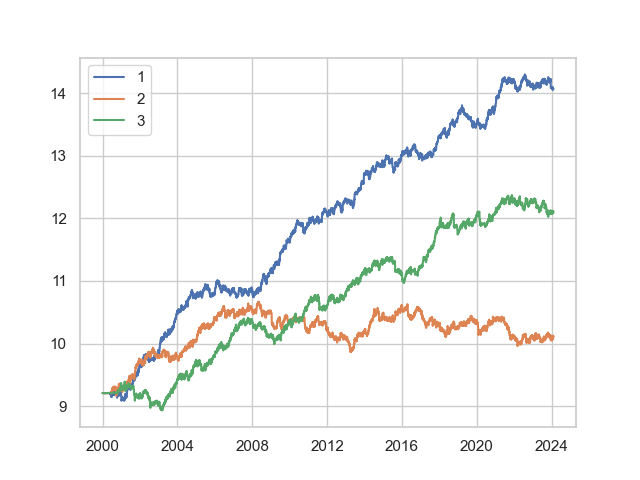
    plt.plot(np.log(df1.capital),label="1")
    plt.plot(np.log(df2.capital),label="2")
    plt.plot(np.log(df3.capital),label="3")
    plt.legend()
    plt.show()
Crypto, Currencies, Fees and Customization
The Alpha library backtesting example from the Backtesting section used daily data, but it is capable of performing backtest logic on finer granularities and on weekends/holidays. If the trading intervals are finer than daily periods, it should also be specified whether trading is around the clock (24 hours, as in currency and crypto) or RTH (6.5 hours standard). This is to adjust the internal accounting for volatility and performance metric computation. Currently, hourly and daily granularities are supported.
We may specify parameters such as the execution fees, commission fees, swap/funding rates, granularity period, portfolio volatility, positional inertia, availability of weekend and around-the-clock trading and starting capital.
We shall demonstrate with examples. To aid us in the data retrieval, we will use our quantpylib.datapoller module. Although we can use str alias d, h to indicate daily and hourly granularities, for clarity, we use quantpylib.standards.Period.
We will use the no-code backtesting discussed in the previous section for brevity, but all the changes apply to both Alpha and GeneticAlpha instances. We will need the following imports:
import pytz
import numpy as np
import matplotlib.pyplot as plt
from datetime import datetime

from quantpylib.standards import Period
from quantpylib.datapoller.master import DataPoller
from quantpylib.simulator.gene import GeneticAlpha
binance client:
keys = {"binance": True}
datapoller = DataPoller(config_keys=keys)
interval = Period.HOURLY

async def main():
    #...examples as before

if __name__ == "__main__":
    import asyncio
    asyncio.run(main())
    example1="ls_10/90(mult(div(minus(low,close),minus(high,low)),div(open,close)))"
    example2="ls_10/90(neg(mean_5(csrank(div(logret_5(),volatility_12())))))"
    example3="mac_50/100(close)"

    period_start = datetime(2010,10,2, tzinfo=pytz.utc)
    period_end = datetime.now(pytz.utc)
    tickers = ["BTCUSDT","ETHUSDT","SOLUSDT"]
    ticker_dfs = [datapoller.crypto.get_trade_bars(
        ticker=ticker,
        start=period_start,
        end=period_end,
        granularity=interval,
        granularity_multiplier=1,
        src="binance"
    ) for ticker in tickers]
    dfs = {ticker:df for ticker,df in zip(tickers,ticker_dfs)}
DataPoller gracefully strings together multiple requests and paces out the requests to get us the required interval data. The specifics of these should be referred to in the quantpylib.datapoller module.
Let us make this fit to the crypto market configuratons and time intervals. We first examine zero-cost performance, specify 24/7 trading and use Period.HOURLY interval. Instead of specifying start and end backtest dates, we can actually let the Alpha engine guess these parameters from the range of the dataframes provided in dfs, if we want the maximum possible range. Other than specifying the config arguments differently, all other code remains the same.
configs={
"dfs":dfs,
"instruments":tickers,
"execrates": [0] * len(tickers),
"longswps": [0] * len(tickers),
"shortswps": [0] * len(tickers),
"granularity": interval,
"around_the_clock":True,
"weekend_trading":True
}
alpha1 = GeneticAlpha(genome=example1,**configs)
alpha2 = GeneticAlpha(genome=example2,**configs)
alpha3 = GeneticAlpha(genome=example3 ,**configs, portfolio_vol=0.10)
df1 = await alpha1.run_simulation()
df2 = await alpha2.run_simulation()
df3 = await alpha3.run_simulation()
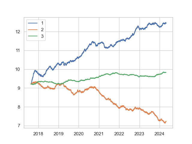
plt.plot(np.log(df1.capital),label="1")
plt.plot(np.log(df2.capital),label="2")
plt.plot(np.log(df3.capital),label="3")
plt.legend()
plt.show()
alpha1 and alpha2 performed reasonably in the crypto markets too.
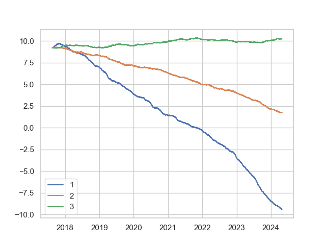
However, for a more realistic modelling, we would need to model the costs of transacting. In practice, we are also unlikely to fully rebalance to the optimal portfolio due to transaction costs. Let us try to take these into consideration.
First, a reasonable execution fee is 0.0003 (this sits slightly higher than the maker-fees for trading USDT perpetuals on Binance for Regular User status). For simplicity, we assume a 10% APR funding rate for perps. To restrict constant rebalancing, we rebalance each position only when held position sits at distance greater than 20% from its optimal position. Let's run a new config:
    configs={
        "dfs":dfs,
        "instruments":tickers,
        "execrates": [0.0003] * len(tickers),
        "longswps": [0.1] * len(tickers), #annualized
        "shortswps": [-0.1] * len(tickers),
        "granularity": interval,
        "around_the_clock":True,
        "weekend_trading":True,
        "positional_inertia": 0.20,
    }

    alpha1 = GeneticAlpha(genome=example1,**configs)
    alpha2 = GeneticAlpha(genome=example2,**configs)
    alpha3 = GeneticAlpha(genome=example3 ,**configs)
    df1 = await alpha1.run_simulation()
    df2 = await alpha2.run_simulation()
    df3 = await alpha3.run_simulation()
    plt.plot(np.log(df1.capital),label="1")
    plt.plot(np.log(df2.capital),label="2")
    plt.plot(np.log(df3.capital),label="3")
    plt.legend()
    plt.show()
Performance Metrics and Hypothesis Tests
Our batteries-included feature gives us an access to powerful statistical tools to evaluate our trading strategy
with a simple function call. This is supported by any BaseAlpha instance, which is indeed sufficed by both Alpha
and GeneticAlpha instances.
async def main():

    '''
    ...
    '''
    print(alpha1.get_performance_measures())
    print(await alpha1.hypothesis_tests())

    print(_alpha1.get_performance_measures())
    print(await _alpha1.hypothesis_tests())
Regression Analysis
In the no-code backtesting, we used quantpylib.simulator.gene.Gene class
functionalities for parsing mathematical/formulaic strings and evaluating them to perform backtest simulations. This parser-evaluator can also be leveraged to provide extremely simple interfaces for powering
regression analysis, as in common-practice in the R, S-like languages. Any regression model involving variables supported by the list-of-primitives can be used. quantpylib.simulator.models features an abstraction layer written on top of this Gene class and statsmodels to perform no-code regression analysis using simple string specifications.
An example scenario for quantitative analysis is a momentum study on the impact of normalized returns on forward one-period daily returns.
Let us take the following setup:import pytz
from datetime import datetime
from quantpylib.standards import Period
from quantpylib.datapoller.master import DataPoller
from quantpylib.simulator.models import GeneticRegression
keys = {"binance":True}
datapoller = DataPoller(config_keys=keys)
interval = Period.DAILY
async def main():
pass
#code here
if __name__ == "__main__":
import asyncio
asyncio.run(main())
    period_start = datetime(2010,1,1, tzinfo=pytz.utc)
    period_end = datetime.now(pytz.utc)
    tickers = ["BTCUSDT","ETHUSDT","BNBUSDT","SOLUSDT","XRPUSDT","DOGEUSDT","ADAUSDT","DOTUSDT","LINKUSDT","MATICUSDT"]
    ticker_dfs = [datapoller.crypto.get_trade_bars(
        ticker=ticker,
        start=period_start,
        end=period_end,
        granularity=interval,
        src="binance"
    ) for ticker in tickers]
    dfs = {ticker:df for ticker,df in zip(tickers,ticker_dfs)}
    configs = {
        "dfs":dfs,
        "instruments":tickers,
        "granularity":interval
    }
GeneticRegression:
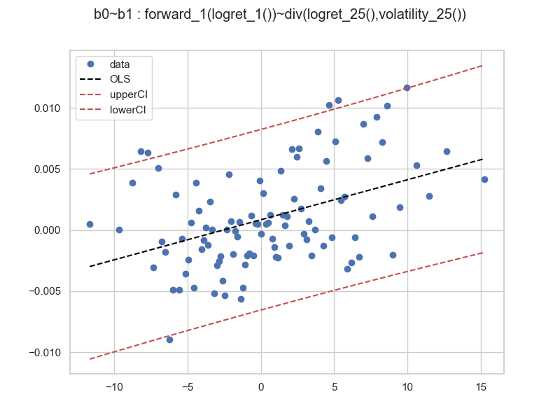
    model = GeneticRegression(
        formula="forward_1(logret_1()) ~ div(logret_25(),volatility_25())",
        **configs
    )
print(model.blockmap) #{'b0': 'forward_1(logret_1())', 'b1': 'div(logret_25(),volatility_25())'}
print(model.smf) #b0~b1
res = model.ols() #statsmodels.regression.linear_model.RegressionResults
print(res.summary())
                            OLS Regression Results
==============================================================================
Dep. Variable:                     b0   R-squared:                       0.001
Model:                            OLS   Adj. R-squared:                  0.001
Method:                 Least Squares   F-statistic:                     28.11
Date:                Wed, 01 May 2024   Prob (F-statistic):           1.16e-07
Time:                        16:48:36   Log-Likelihood:                 28193.
No. Observations:               19648   AIC:                        -5.638e+04
Df Residuals:                   19646   BIC:                        -5.637e+04
Df Model:                           1
Covariance Type:            nonrobust
==============================================================================
                 coef    std err          t      P>|t|      [0.025      0.975]
------------------------------------------------------------------------------
Intercept      0.0011      0.000      2.567      0.010       0.000       0.002
b1             0.0004   7.73e-05      5.301      0.000       0.000       0.001
==============================================================================
Omnibus:                     8766.454   Durbin-Watson:                   1.010
Prob(Omnibus):                  0.000   Jarque-Bera (JB):          1610674.284
Skew:                           1.041   Prob(JB):                         0.00
Kurtosis:                      47.307   Cond. No.                         5.37
==============================================================================
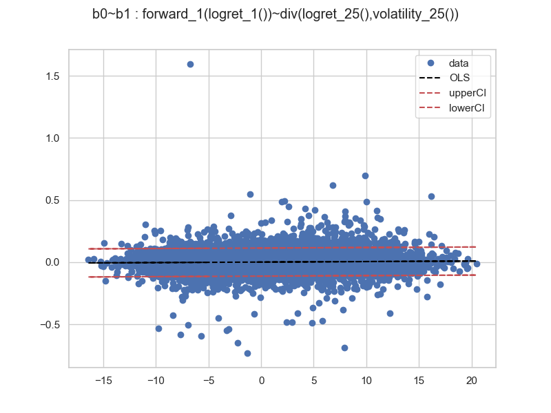
and a leverage plot:
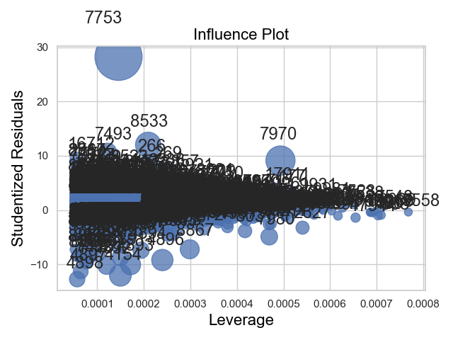
We see that the although we had strong outliers in the standardized residuals, those with extreme residuals tended to have lower leverage values w.r.t the regressor variable hull. We had 19648 observations for the regression, hence the influence plots and other diagnostics may be difficult to interpret. Also, the leverage values indicate how much the model fit depends on these outlier points, but we would like to see for ourself how the models perform when extremes are smoothed/muted out.
We also want to create more interpretive analysis and plots. The ols method takes in
the number of bins, the block identifier to bin by, bin-method and aggregating method. By default, the binning is done on the response variable axis b0, and binned by equal observation-cardinality intervals. The aggregator defaults to the 0.05-quantile-winsorized-means on both tails, to mute tails common in market contexts.
For our sceneario, let us take 100 bins over the b1 axis, which is our normalized returns,
and take the remaining default options.
                            OLS Regression Results
==============================================================================
Dep. Variable:                     b0   R-squared:                       0.184
Model:                            OLS   Adj. R-squared:                  0.176
Method:                 Least Squares   F-statistic:                     22.11
Date:                Wed, 01 May 2024   Prob (F-statistic):           8.45e-06
Time:                        18:03:49   Log-Likelihood:                 418.85
No. Observations:                 100   AIC:                            -833.7
Df Residuals:                      98   BIC:                            -828.5
Df Model:                           1
Covariance Type:            nonrobust
==============================================================================
                 coef    std err          t      P>|t|      [0.025      0.975]
------------------------------------------------------------------------------
Intercept      0.0008      0.000      2.259      0.026       0.000       0.002
b1             0.0003   6.98e-05      4.702      0.000       0.000       0.000
==============================================================================
Omnibus:                        4.233   Durbin-Watson:                   1.528
Prob(Omnibus):                  0.120   Jarque-Bera (JB):                4.101
Skew:                           0.444   Prob(JB):                        0.129
Kurtosis:                       2.559   Cond. No.                         5.36
==============================================================================

Notes:
[1] Standard Errors assume that the covariance matrix of the errors is correctly specified.
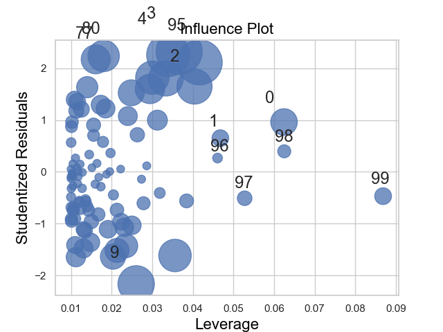
and all regression studies suggest that momentum exists in cryptocurrency returns over daily timescales. Of course, since the data has been transformed, the interpretation of the regression results and analysis needs to be adjusted in relation to the binning and aggregation techniques employed.
The library also supports methods to study multivariable regression, as in the statsmodels package, as well as convenience methods to obtain diagnostics for common issues such as multicollinearity concerns with statistics like condition number and variance-inflation-factors.